4. Double counterfactual prediction
4.1. We will be performing a double counterfactual prediction in this tutorial, recreating the CellDISECT results from benchmarking scenario 2 of the paper on the Eraslan et al. data.
[1]:
# enable autoreload
%load_ext autoreload
%autoreload 2
%matplotlib inline

import os
import random

import scvi
scvi.settings.seed = 0
import scanpy as sc
import anndata as ad
import torch
import numpy as np
import pandas as pd
import gc
import scipy
from scipy.stats import pearsonr
from scipy.stats import wasserstein_distance
torch.set_float32_matmul_precision('medium')
import matplotlib.pyplot as plt
from matplotlib.pyplot import rc_context
import seaborn as sns

import warnings
from tqdm import tqdm
warnings.simplefilter("ignore", UserWarning)
warnings.filterwarnings("ignore")


from celldisect import CellDISECT
Global seed set to 0
Global seed set to 0
[2]:
RANDOM_SEED = 42

adata = sc.read_h5ad('/lustre/scratch126/cellgen/team205/aa34/Arian/Dis2P/eraslan_preprocessed1212_split_deg.h5ad')
adata = adata[adata.layers['counts'].sum(1) != 0].copy()
if scipy.sparse.issparse(adata.X):
    adata.X = adata.X.todense()
if scipy.sparse.issparse(adata.layers['counts']):
    adata.layers['counts'] = adata.layers['counts'].todense()

adata.X = adata.layers['counts'].copy()

cats = ['tissue', 'Sample ID', 'sex', 'Age_bin']
[3]:
cell_type_included = False # Set to True if you have provided a cell type annotation in the cats list

if not cell_type_included:
    adata.obs["_cluster"] = (
        "0"  # Dummy obs for inference (not-training) time, to avoid computing neighbors and clusters again in setup_anndata | AVOID ADDING BEFORE TRAINING
    )
[4]:
n_samples_from_source_max = 500
4.2. We have already trained the model without cell type information using the default parameters as in the example:
https://github.com/Lotfollahi-lab/CellDISECT/blob/main/examples/training_example.py
[5]:
pre_path = '/lustre/scratch126/cellgen/team205/aa34/Arian/Dis2P/models/'

split_name = 'split_2'
gc.collect()

celldisect_model_path = (
    f'dis2p_cE_{split_name}/'
f'pretrainAE_0_maxEpochs_1000_split_{split_name}_reconW_20_cfWeight_0.8_beta_0.003_clf_0.05_adv_0.014_advp_5_n_cf_1_lr_0.003_wd_5e-05_new_cf_True_dropout_0.1_n_hidden_128_n_latent_32_n_layers_2batch_size_256_NoCT'
)

model = CellDISECT.load(f"{pre_path}/{celldisect_model_path}", adata=adata)
INFO     File
         /lustre/scratch126/cellgen/team205/aa34/Arian/Dis2P/models//dis2p_cE_split_2/pretrainAE_0_maxEpochs_1000_s
         plit_split_2_reconW_20_cfWeight_0.8_beta_0.003_clf_0.05_adv_0.014_advp_5_n_cf_1_lr_0.003_wd_5e-05_new_cf_T
         rue_dropout_0.1_n_hidden_128_n_latent_32_n_layers_2batch_size_256_NoCT/model.pt already downloaded
Cluster covariate already present in adata.obs, remove in case you want to re-run, skipping!
4.3. We are aiming to predict, what would Epithelial female breast cells look like, given if they were male prostate gland cells.
4.3.1. So this is a double counterfactual, aiming to change 2 of the covariates at the same time in the cells, sex, and tissue in this case.
We are also using just the Epithelial subset of the dataset, since we want to do the counterfactuals on this group of cells. You can take a look at the documentation of the predict_counterfactuals method for more details.
[6]:
cell_type_to_check = 'Epithelial cell (luminal)'
n_samples_from_source = min(n_samples_from_source_max, len(adata[(adata.obs['Broad cell type'] == cell_type_to_check) &
                (adata.obs['tissue'] == 'breast') & (adata.obs['sex'] == 'female')]))


cov_names = ['sex', 'tissue']
cov_values = ['female', 'breast']
cov_values_cf = ['male', 'prostate gland']

adata_ = adata[adata.obs['Broad cell type'] == cell_type_to_check].copy()
[7]:
x_ctrl, x_true, x_pred = model.predict_counterfactuals(
                                        adata_,
                                        cov_names=cov_names,
                                        cov_values=cov_values,
                                        cov_values_cf=cov_values_cf,
                                        cats=cats,
                                        n_samples_from_source=n_samples_from_source,
                                        seed=RANDOM_SEED,
                                        )

x_ctrl, x_true, x_pred = np.log1p(x_ctrl), np.log1p(x_true), np.log1p(x_pred)
INFO     AnnData object appears to be a copy. Attempting to transfer setup.
INFO     AnnData object appears to be a copy. Attempting to transfer setup.
The predict_counterfactuals method gave us the control cells (female breast), true cells (actual male prostate), and CellDISECT's prediction of female breast --> male prostate as output.
We have the differentially expressed genes related to this transformation precomputed. You can compute these genes with the code in the following notebook: https://github.com/stathismegas/CellDISECT_reproducibility/blob/main/figure_notebooks/eraslan/eraslan_preprocess_scenario_splits.ipynb
[8]:
deg_list = adata.uns['rank_genes_groups_split_2']['male_prostate gland']
[9]:
deg_list
[9]:
array(['KLK4', 'AC005152.3', 'LINC01152', 'HP', 'CD177', 'KLK3',
       'PLA2G2A', 'XIST', 'KLK2', 'CPLX3', 'NKX3-1', 'RP11-395B7.2',
       'MSMB', 'ATOH8', 'ACPP', 'MT1G', 'S100P', 'ANKRD30A', 'NEFH',
       'IFI6', 'PCAT4', 'PGC', 'FTL', 'SLC45A3', 'CKB', 'GP2',
       'LINC01297', 'SLC38A11', 'MT1M', 'RPS4Y1', 'FGL1', 'RP1-288H2.2',
       'PLPP1', 'SORD', 'AKAP12', 'CYP1B1', 'SFN', 'ADIRF', 'CPNE4',
       'GPX3', 'UBA52', 'TIMP1', 'KIT', 'TMEFF2', 'TRPM8', 'ATP5E',
       'GABRP', 'HSPA1A', 'STAC2', 'UQCR10', 'MT2A', 'HERPUD1', 'S100A11',
       'SCD', 'RP11-33A14.1', 'SLC4A4', 'MT1E', 'PSCA', 'RP11-126O1.4',
       'UBB', 'VTCN1', 'IFITM3', 'AGR2', 'SCNN1G', 'TMSB10', 'NDUFA4',
       'SCHLAP1', 'AMD1', 'B2M', 'NDRG1', 'PSAP', 'KRT15', 'RP11-384F7.2',
       'STEAP2', 'CPE', 'COX7C', 'FAU', 'PRDX1', 'AQP3', 'ALOX15B',
       'GADD45G', 'SHROOM1', 'SERF2', 'LSAMP', 'DHCR24', 'UQCRB', 'ZNF90',
       'C19orf48', 'POLR2L', 'COX6B1', 'CST3', 'TXNRD1', 'ESR1', 'OOEP',
       'HGD', 'TPT1', 'NDUFS5', 'TSPO', 'AC009478.1', 'RNF19B', 'PART1',
       'UQCRQ', 'FN1', 'APOO', 'MTRNR2L8', 'ANKRD36C', 'BARX2',
       'RP11-356O9.1', 'COX5B', 'FOLH1', 'FXYD3', 'BMPR1B', 'TMPRSS2',
       'SYNM', 'DHFR', 'FADS2', 'TBC1D3P1-DHX40P1', 'CSTB', 'SEPW1',
       'GAPDH', 'SYT1', 'SERPINA3', 'EEF1A1', 'H2AFJ', 'ALDOA',
       'RP11-608O21.1', 'GABRG3', 'ATP5L', 'ADAMTS9', 'CRISPLD1', 'PFN1',
       'GRM7', 'RP11-368L12.1', 'GRN', 'FTH1', 'SDC1', 'SELM', 'DBI',
       'COX7A2', 'TACSTD2', 'PPDPF', 'CYP4F22', 'C14orf2', 'ALDH1A2',
       'UQCRH', 'COX4I1', 'MTRNR2L12', 'SOD2', 'PDE11A', 'PRUNE2', 'PDK4',
       'ARHGAP40', 'PERP', 'XPO5', 'CTSB', 'ACTG1', 'PI15', 'RNF144B',
       'GLUL', 'CACNA1C', 'KRT19', 'SLC39A6', 'LMO7', 'FASN', 'SPDEF',
       'BAIAP2L1', 'ACSM3', 'TMEM178B', 'CACNB2', 'TFCP2L1', 'ELF3',
       'MGP', 'MYL6', 'MRPL41', 'ESRRG', 'KRT7', 'THBS1', 'MBOAT2',
       'CD24', 'AC072062.1', 'PLEKHA7', 'HSPB1', 'AZGP1', 'CLDN4', 'DSP',
       'TTC6', 'SOX4', 'PLAT', 'XBP1', 'MYBPC1', 'HS3ST4', 'DSTN',
       'SPINT1', 'AIM1', 'HES1', 'CPEB4', 'ACTB', 'RBPJ', 'SORBS2',
       'RASGEF1B'], dtype=object)
4.4. Earth Mover’s Distance metric on 20 DEGs and all genes
[13]:
emd_results = {}
for n_top_deg in [20, None]:
    if n_top_deg is not None:
        degs = np.where(np.isin(adata.var_names, deg_list[:n_top_deg]))[0]
    else:
        degs = np.arange(adata.n_vars)
        n_top_deg = 'all'

    x_true_deg = x_true[:, degs]
    x_pred_deg = x_pred[:, degs]
    x_ctrl_deg = x_ctrl[:, degs]

    emd_results[str(n_top_deg)] = {}
    for method_name, method in zip(['CellDISECT', 'Control'], [x_pred_deg, x_ctrl_deg]):
        wd = []
        for i in range(x_true_deg.shape[1]):
            wd.append(
                wasserstein_distance(torch.tensor(x_true_deg[:, i]), torch.tensor(method[:, i]))
            )
        emd_results[str(n_top_deg)][method_name] = np.mean(wd)

emd_results = pd.DataFrame.from_dict(emd_results).T
emd_results
[13]:
| CellDISECT | Control | |
|---|---|---|
| 20 | 0.506272 | 0.636810 |
| all | 0.108333 | 0.088362 |
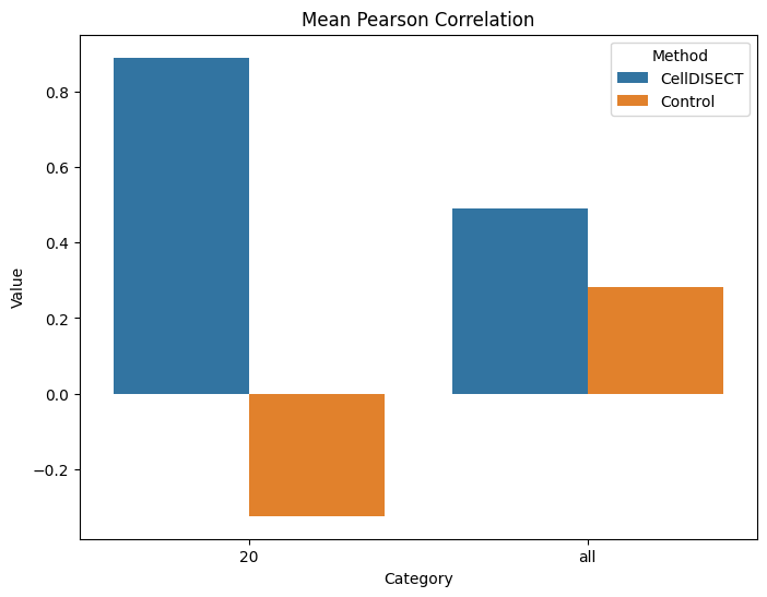
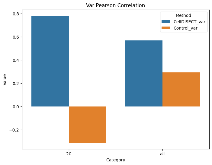
4.5. Pearson Correlation metric on 20 DEGs and all genes
[15]:
r2_results = {}
for n_top_deg in [20, None]:
    if n_top_deg is not None:
        degs = np.where(np.isin(adata.var_names, deg_list[:n_top_deg]))[0]
    else:
        degs = np.arange(adata.n_vars)
        n_top_deg = 'all'

    x_true_deg = x_true[:, degs]
    x_pred_deg = x_pred[:, degs]
    x_ctrl_deg = x_ctrl[:, degs]


    r2_mean_deg = pearsonr(x_true_deg.mean(0), x_pred_deg.mean(0))
    r2_mean_base_deg = pearsonr(x_true_deg.mean(0), x_ctrl_deg.mean(0))

    r2_var_deg = pearsonr(x_true_deg.var(0), x_pred_deg.var(0))
    r2_var_base_deg = pearsonr(x_true_deg.var(0), x_ctrl_deg.var(0))

    r2_results[str(n_top_deg)] = {}
    r2_results[str(n_top_deg)]['CellDISECT'] = r2_mean_deg[0]
    r2_results[str(n_top_deg)]['Control'] = r2_mean_base_deg[0]

    r2_results[str(n_top_deg)]['CellDISECT_var'] = r2_var_deg[0]
    r2_results[str(n_top_deg)]['Control_var'] = r2_var_base_deg[0]

r2_results = pd.DataFrame.from_dict(r2_results).T
r2_results
[15]:
| CellDISECT | Control | CellDISECT_var | Control_var | |
|---|---|---|---|---|
| 20 | 0.889936 | -0.323958 | 0.780835 | -0.311901 |
| all | 0.490695 | 0.282120 | 0.568846 | 0.292532 |
[23]:
df_long = r2_results[['CellDISECT', 'Control']].reset_index().melt(id_vars='index',
                                       var_name='Method',
                                       value_name='Value')
df_long.rename(columns={'index': 'Category'}, inplace=True)

# Create the grouped barplot
plt.figure(figsize=(8, 6))
sns.barplot(data=df_long, x='Category', y='Value', hue='Method')

# Customize the plot
plt.title("Mean Pearson Correlation")
plt.ylabel('Value')

# Show the plot
plt.show()

df_long = r2_results[['CellDISECT_var', 'Control_var']].reset_index().melt(id_vars='index',
                                       var_name='Method',
                                       value_name='Value')
df_long.rename(columns={'index': 'Category'}, inplace=True)

# Create the grouped barplot
plt.figure(figsize=(8, 6))
sns.barplot(data=df_long, x='Category', y='Value', hue='Method')

# Customize the plot
plt.title("Var Pearson Correlation")
plt.ylabel('Value')

# Show the plot
plt.show()
4.6. Delta Pearson Correlation metric on 20 DEGs and all genes
[16]:
r2_results_subtract = {}
for n_top_deg in [20, None]:
    if n_top_deg is not None:
        degs = np.where(np.isin(adata.var_names, deg_list[:n_top_deg]))[0]
    else:
        degs = np.arange(adata.n_vars)
        n_top_deg = 'all'

    x_true_deg = x_true[:, degs]
    x_pred_deg = x_pred[:, degs]
    x_ctrl_deg = x_ctrl[:, degs]


    r2_mean_deg = pearsonr(x_true_deg.mean(0) - x_ctrl_deg.mean(0), x_pred_deg.mean(0) - x_ctrl_deg.mean(0))

    r2_var_deg = pearsonr(x_true_deg.var(0) - x_ctrl_deg.var(0), x_pred_deg.var(0) - x_ctrl_deg.var(0))

    r2_results_subtract[str(n_top_deg)] = {}
    r2_results_subtract[str(n_top_deg)]['CellDISECT'] = r2_mean_deg[0]

    r2_results_subtract[str(n_top_deg)]['CellDISECT_var'] = r2_var_deg[0]

r2_results_subtract = pd.DataFrame.from_dict(r2_results_subtract).T
r2_results_subtract
[16]:
| CellDISECT | CellDISECT_var | |
|---|---|---|
| 20 | 0.729744 | 0.641065 |
| all | 0.400509 | 0.151026 |