3. Flexible fairness for batch correction
3.1. Latent combination tutorial for erythroid organ inference
3.1.1. The model that will be loaded in the following cells, has been trained on the Suo et al. dataset using the following script:
[1]:
# enable autoreload
%load_ext autoreload
%autoreload 2
%matplotlib inline

import os
import random

import scvi
scvi.settings.seed = 0
import scanpy as sc
import anndata as ad
import torch
import numpy as np
import pandas as pd
import gc
torch.set_float32_matmul_precision('medium')
import matplotlib.pyplot as plt
from matplotlib.pyplot import rc_context
import seaborn as sns

import warnings
from tqdm import tqdm
warnings.simplefilter("ignore", UserWarning)
warnings.filterwarnings("ignore")

from celldisect import CellDISECT
Global seed set to 0
Global seed set to 0
[2]:
data_path = '/lustre/scratch126/cellgen/team205/aa34/Arian/Dis2P/dis2p_reproducibility/figure_notebooks/antony/suo_prep_data.h5ad'

adata = sc.read_h5ad(data_path)
adata.X = adata.layers['counts'].copy()
adata = adata[adata.X.sum(1) != 0].copy()
adata.var['highly_variable'] = adata.var['highly_variable'].astype(bool)

cats = ['integration_donor', 'integration_library_platform_coarse',
        'organ']
cell_type_included = False # Set to True if you have provided a cell type annotation in the cats list

if not cell_type_included:
    adata.obs["_cluster"] = (
        "0"  # Dummy obs for inference (not-training) time, to avoid computing neighbors and clusters again in setup_anndata | AVOID ADDING BEFORE TRAINING
    )
adata
[2]:
AnnData object with n_obs × n_vars = 841966 × 8192
    obs: 'study', 'sample_ID', 'lane_ID', 'organ', 'age', 'cell_type', 'sex', 'sex_inferred', 'sample_status', 'library_platform', 'strand_sequence', 'biological_unit', 'doi', 'institute', 'study_PI', 'subject_ID', 'ethnicity_1', 'ethnicity_2', 'disease_known', 'disease_condition', 'subject_type', 'sample_type', 'sample_cultured', 'anatomical_region', 'anatomical_region_level_2', 'protocol_tissue_dissociation', 'cell_enrichment', 'reference_genome', 'reference_genome_ensembl_release', 'reads_processing', 'sequencing_platform', 'Sample_orig_author', 'Anatomical_region_orig_author', 'Termination_method_orig_author', 'Method_orig_author', 'anno_lvl_2_final_clean_orig_author', 'integration_donor', 'integration_biological_unit', 'integration_sample_status', 'integration_library_platform_coarse', 'author_batch', 'Chuan_meta_Original_Label', 'Chuan_meta_Harmonised_Label', 'Chuan_meta_Tissue', 'Chuan_meta_Technology', 'Chuan_meta_Donor', 'Chuan_meta_Age', 'orig_anno', 'trimester', 'bin_age', '_cluster', '_scvi_batch', '_scvi_labels', '_scvi_cluster'
    var: 'GeneID', 'GeneName', 'n_counts', 'highly_variable', 'means', 'dispersions', 'dispersions_norm'
    uns: '_scvi_manager_uuid', '_scvi_uuid', 'bin_age_colors', 'cell_type_colors', 'hvg', 'integration_donor_colors', 'integration_library_platform_coarse_colors', 'log1p', 'organ_colors'
    obsm: '_scvi_extra_categorical_covs'
    layers: 'counts'
[3]:
pd.set_option('display.max_rows', 500)

adata.obs['orig_anno'].value_counts()
[3]:
orig_anno
MID_ERY                                  55104
MACROPHAGE_IRON_RECYCLING                48640
MACROPHAGE_LYVE1_HIGH                    35001
NK                                       30284
FIBROBLAST_VII                           30142
FIBROBLAST_I                             25041
DP(P)_T                                  22839
FIBROBLAST_IV                            22634
YS_ERY                                   20370
MATURE_B                                 17489
MACROPHAGE_MHCII_HIGH                    14872
MACROPHAGE_PROLIFERATING                 14391
DN(Q)_T                                  13655
CD4+T                                    13649
FIBROBLAST_VIII                          12719
ENDOTHELIUM_IV                           12601
DP(Q)_T                                  12390
EARLY_ERY                                11897
MONOCYTE_I_CXCR4                         11891
DC2                                      11491
FIBROBLAST_X                             11415
MYOFIBROBLAST                            11238
FIBROBLAST_II                            10984
LATE_ERY                                 10814
MONOCYTE_II_CCR2                         10660
LARGE_PRE_B                              10468
PROMONOCYTE                               9866
DN(P)_T                                   9810
ENDOTHELIUM_III                           9416
CD8+T                                     9369
EPITHELIUM_II                             9155
ENDOTHELIUM_I                             8972
FIBROBLAST_XI                             8864
MONOCYTE_III_IL1B                         8675
SMALL_PRE_B                               8263
PRO_B                                     8113
CYCLING_EPITHELIUM                        7881
CYCLING_FIBROBLAST_I                      7870
HEPATOCYTE_II                             7845
CYCLING_FIBROBLAST_II                     7770
ABT(ENTRY)                                7066
CYCLING_NK                                7052
TREG                                      6850
LATE_PRO_B                                6340
MUSCLE_SATELLITE                          6041
ILC3                                      5931
EARLY_MK                                  5831
MEP                                       5729
DEVELOPING_NEPHRON_I                      5727
TYPE_1_INNATE_T                           5727
B1                                        5652
FIBROBLAST_V                              5564
MYOFIBROBLAST_I                           5562
LATE_MK                                   5472
FIBROBLAST_XIV                            5333
MACROPHAGE_KUPFFER_LIKE                   5214
CD8AA                                     4737
FIBROBLAST_III                            4569
FIBROBLAST_VI                             4300
GMP                                       3995
CYCLING_DC                                3908
MAST_CELL                                 3897
HSC_MPP                                   3816
MOP                                       3753
CYCLING_YS_ERY                            3516
MACROPHAGE_ERY                            3302
FIBROBLAST_IX                             3286
DC1                                       3138
PROMYELOCYTE                              3113
PRE_PRO_B                                 3034
TYPE_3_INNATE_T                           3031
CYCLING_T                                 2985
SMOOTH_MUSCLE                             2912
FIBROBLAST_XIII                           2892
FIBROBLAST_XV                             2804
FIBROBLAST_XII                            2719
IMMATURE_B                                2689
EPITHELIUM_I                              2597
CMP                                       2579
HEPATOCYTE_I                              2561
PDC                                       2473
CYCLING_MPP                               2440
FIBROBLAST_XVII                           2342
EOSINOPHIL_BASOPHIL                       2334
MEMP                                      2238
HEPATOCYTE-LIKE                           2224
KERATINOCYTE                              2151
NEURON                                    2010
CYCLING_B                                 1909
DEVELOPING_NEPHRON_II                     1749
OSTEOBLAST                                1734
DN(early)_T                               1670
LMPP_MLP                                  1395
MACROPHAGE_PERI                           1301
ENDOTHELIUM_II                            1244
OSTEOCLAST                                1199
NEUTROPHIL                                1075
MESOTHELIUM                               1039
MYELOCYTE                                 1019
CYCLING_MEMP                               922
MELANOCYTE                                 899
MACROPHAGE_TREM2                           888
ENDOTHELIUM_V                              809
CYCLING_ILC                                541
CYCLING_PDC                                532
ENTEROENDOCRINE_I                          503
ILC2                                       468
MIGRATORY_DC                               421
INTERSTITIAL_CELLS_OF_CAJAL                409
YS_STROMA                                  334
MESENCHYMAL_LYMPHOID_TISSUE_ORGANISER      300
AS_DC                                      266
CHONDROCYTE                                253
ENTEROENDOCRINE_II                         231
PRE_DC2                                    215
FIBROBLAST_XVI                             207
DC_PROGENITOR                              200
SKELETAL_MUSCLE                            123
LANGERHANS_CELLS                            66
PLASMA_B                                    61
Name: count, dtype: int64
[4]:
celltypes = [
'MID_ERY',
'EARLY_ERY',
'LATE_ERY',
'HSC_MPP',
'MEMP',
'CYCLING_MEMP',
'MEP',
]
[5]:
adata = adata[adata.obs['orig_anno'].isin(celltypes)].copy()
[6]:
module_name = f'Antony_suoFull_NoAge'
pre_path = f'/lustre/scratch126/cellgen/team205/aa34/Arian/Dis2P/models/{module_name}'
model_name = 'development_clustering_pretrainAE_0_maxEpochs_1000_reconW_20_cfWeight_0.8_beta_0.003_clf_0.02_adv_0.014_advp_5_n_cf_1_lr_0.003_wd_5e-05_new_cf_True_dropout_0.1_n_hidden_128_n_latent_32_n_layers_2_weighted_classifier_False'

model = CellDISECT.load(f"{pre_path}/{model_name}", adata=adata)
INFO     File
         /lustre/scratch126/cellgen/team205/aa34/Arian/Dis2P/models/Antony_suoFull_NoAge/development_clustering_pre
         trainAE_0_maxEpochs_1000_reconW_20_cfWeight_0.8_beta_0.003_clf_0.02_adv_0.014_advp_5_n_cf_1_lr_0.003_wd_5e
         -05_new_cf_True_dropout_0.1_n_hidden_128_n_latent_32_n_layers_2_weighted_classifier_False/model.pt already
         downloaded
Cluster covariate already present in adata.obs, remove in case you want to re-run, skipping!
[7]:
adata
[7]:
AnnData object with n_obs × n_vars = 90520 × 8192
    obs: 'study', 'sample_ID', 'lane_ID', 'organ', 'age', 'cell_type', 'sex', 'sex_inferred', 'sample_status', 'library_platform', 'strand_sequence', 'biological_unit', 'doi', 'institute', 'study_PI', 'subject_ID', 'ethnicity_1', 'ethnicity_2', 'disease_known', 'disease_condition', 'subject_type', 'sample_type', 'sample_cultured', 'anatomical_region', 'anatomical_region_level_2', 'protocol_tissue_dissociation', 'cell_enrichment', 'reference_genome', 'reference_genome_ensembl_release', 'reads_processing', 'sequencing_platform', 'Sample_orig_author', 'Anatomical_region_orig_author', 'Termination_method_orig_author', 'Method_orig_author', 'anno_lvl_2_final_clean_orig_author', 'integration_donor', 'integration_biological_unit', 'integration_sample_status', 'integration_library_platform_coarse', 'author_batch', 'Chuan_meta_Original_Label', 'Chuan_meta_Harmonised_Label', 'Chuan_meta_Tissue', 'Chuan_meta_Technology', 'Chuan_meta_Donor', 'Chuan_meta_Age', 'orig_anno', 'trimester', 'bin_age', '_cluster', '_scvi_batch', '_scvi_labels', '_scvi_cluster'
    var: 'GeneID', 'GeneName', 'n_counts', 'highly_variable', 'means', 'dispersions', 'dispersions_norm'
    uns: '_scvi_manager_uuid', '_scvi_uuid', 'bin_age_colors', 'cell_type_colors', 'hvg', 'integration_donor_colors', 'integration_library_platform_coarse_colors', 'log1p', 'organ_colors'
    obsm: '_scvi_extra_categorical_covs'
    layers: 'counts'
3.3. You can also use the combination of covariates/latents as you like, here we are using a combination/concatenation of Z0 with each of the covariates to make new latents Z0+ZCov
[9]:
# Z_{0+Z_i} = Z_0 + Z_i | Optional
# This represents the combination of latents with Z_0.
# Here, Z_i is a vector where all elements are zero except for the i-th section.
# Z_0 is [latent_0, 0, ..., 0] and Z_i is [0, ..., 0, latent_i, 0, ..., 0].
# When mixing two latents, it will look like [latent_0, 0, latent_i, 0, ..., 0].
for i in range(len(cats)):  # loop over all Z_i
    label = cats[i]
    latent_name = f"CellDISECT_Z_0+{label}"
    adata.obsm[latent_name] = (
        adata.obsm["CellDISECT_Z_0"].copy() + adata.obsm[f"CellDISECT_Z_{label}"].copy()
    )
3.3.1. With the same pattern as above, you can mix any combination of covariates and latents of your choosing:
[10]:
latent_to_make = ['0', 'organ', 'integration_donor']
# or
# latent_to_make = ['organ', 'integration_donor']
# or any other combination
latent_name = "CellDISECT_Z_" + "_".join(latent_to_make)
temp_latent = np.zeros_like(adata.obsm["CellDISECT_Z_0"])
for name in latent_to_make:
    temp_latent += adata.obsm[f"CellDISECT_Z_{name}"].copy()

adata.obsm[latent_name] = (
    temp_latent.copy()
)
del temp_latent
[11]:
latent_name
[11]:
'CellDISECT_Z_0_organ_integration_donor'
You can see that the latent for CellDISECT_Z_0_organ_integration_donor, has the latent vectors in their respective indices, and zeros in the integration_library_platform_coarse indices which was not selected
[12]:
adata.obsm[latent_name][:, :128].sum(0)
[12]:
array([-1.75040391e+04, -3.38555938e+04, -1.87798398e+04,  9.55953320e+03,
        4.61457773e+04,  9.14440703e+04,  7.54916064e+03, -2.18722375e+05,
       -4.83425273e+04, -1.10249328e+05,  3.78672344e+04, -1.38188877e+04,
        3.27485781e+04,  3.94175098e+03,  3.88769375e+04,  5.67719922e+04,
        1.08032750e+05, -2.51776611e+02,  1.60374854e+04, -6.89519688e+04,
        3.04145332e+04, -5.89433750e+04, -5.21918789e+04, -3.42050547e+04,
       -1.01287549e+04,  5.39129736e+03, -1.24341914e+05,  1.29704133e+05,
       -1.53636025e+04,  4.29150156e+04,  5.20313281e+04,  1.09389268e+04,
       -4.40014404e+02,  8.01885437e+02,  9.21002930e+02, -5.22604102e+03,
       -1.21806416e+04,  1.41498975e+03, -5.41523389e+03,  2.66045868e+02,
       -1.32705566e+03, -1.68192981e+03, -2.51068730e+04, -1.28214954e+03,
       -1.68837540e+02,  4.64866914e+04, -2.78392749e+03,  7.40726547e+01,
        9.00216614e+02,  3.55316382e+03, -1.16640845e+03,  2.92287988e+03,
       -4.66438330e+03,  2.16277206e+02,  3.64461680e+04,  8.10476406e+04,
        5.75590703e+04, -2.93583081e+03, -7.71643982e+02,  1.16263086e+04,
        9.97728882e+02,  1.84864197e+03, -6.83654297e+04,  1.75080429e+02,
        0.00000000e+00,  0.00000000e+00,  0.00000000e+00,  0.00000000e+00,
        0.00000000e+00,  0.00000000e+00,  0.00000000e+00,  0.00000000e+00,
        0.00000000e+00,  0.00000000e+00,  0.00000000e+00,  0.00000000e+00,
        0.00000000e+00,  0.00000000e+00,  0.00000000e+00,  0.00000000e+00,
        0.00000000e+00,  0.00000000e+00,  0.00000000e+00,  0.00000000e+00,
        0.00000000e+00,  0.00000000e+00,  0.00000000e+00,  0.00000000e+00,
        0.00000000e+00,  0.00000000e+00,  0.00000000e+00,  0.00000000e+00,
        0.00000000e+00,  0.00000000e+00,  0.00000000e+00,  0.00000000e+00,
        7.52727832e+03,  5.47131836e+03,  1.43137451e+04,  3.71644946e+03,
        3.35054844e+04, -4.50400156e+04,  1.40292125e+05, -7.29384062e+04,
       -9.61884766e+03, -3.87217432e+03, -5.54280090e+02, -4.60546289e+03,
        2.69948164e+04, -5.79350049e+03,  6.75064648e+03, -9.11916309e+03,
        3.27080322e+03,  6.99119688e+04,  8.06322021e+03,  8.51738770e+03,
        3.85352148e+04,  4.99245020e+03,  1.32849082e+04,  6.24061914e+04,
       -3.24508887e+04, -7.79491016e+03,  7.29276719e+04, -5.01927124e+02,
       -2.96022344e+04, -7.79007568e+03,  6.99948145e+03,  5.96621367e+04],
      dtype=float32)
[13]:
cats
[13]:
['integration_donor', 'integration_library_platform_coarse', 'organ']
We are computing the neighbors and umaps for each of these latents, the first loop computes these for Z_0 and Z_organ, and the second look does it for Z_0+organ. (You can loop over all covariates, we hardcoded these 2 latents here ([0, 3]) for faster computation.
[14]:
# Compute neighbors and UMAPs for the latent representations (this might take a while, consider running it using RAPIDS scanpy with a GPU if data is large)
for i in [0, 3]:  # loop over Z_0 and Z_organ | Neighbors and UMAPs for Z_0 and Z_organ
    if i == 0:
        latent_name = f"CellDISECT_Z_{i}"
    else:
        label = cats[i - 1]
        latent_name = f"CellDISECT_Z_{label}"

    latent = ad.AnnData(X=adata.obsm[f"{latent_name}"], obs=adata.obs)
    sc.pp.neighbors(adata=latent, use_rep="X")
    sc.tl.umap(adata=latent)

    adata.uns[f"{latent_name}_neighbors"] = latent.uns["neighbors"]
    adata.obsm[f"{latent_name}_umap"] = latent.obsm["X_umap"]
    gc.collect()

for i in [2]:  # loop over Z_organ | Neighbors and UMAPs for Z_0+Z_organ | Optional
    label = cats[i]
    latent_name = f"CellDISECT_Z_0+{label}"

    latent = ad.AnnData(X=adata.obsm[f"{latent_name}"], obs=adata.obs)
    sc.pp.neighbors(adata=latent, use_rep="X")
    sc.tl.umap(adata=latent)

    adata.uns[f"{latent_name}_neighbors"] = latent.uns["neighbors"]
    adata.obsm[f"{latent_name}_umap"] = latent.obsm["X_umap"]
    gc.collect()
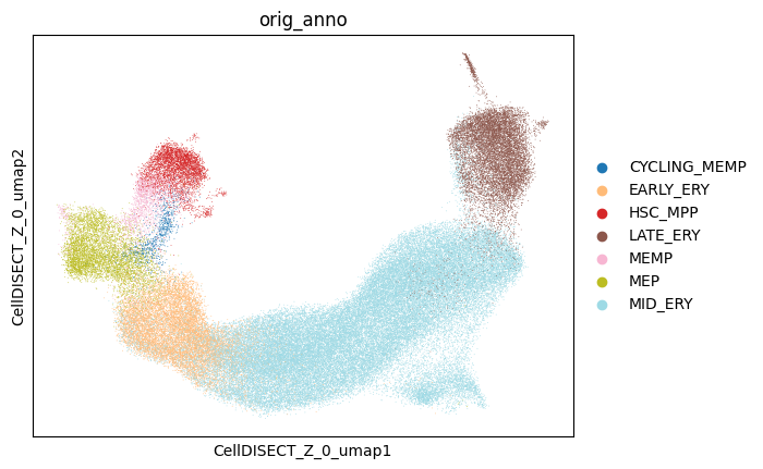
You can see the separation of cell types in Z0 since it was not provided as a covariate and CellDISECT has learnt it unsupervised
[15]:
fig, ax = plt.subplots(nrows=1, ncols=1)
sc.pl.embedding(
    adata,
    basis='CellDISECT_Z_0_umap',
    color='orig_anno',
    groups=celltypes,
    palette='tab20',
    ax=ax,
    show=False,
)

# fig.savefig('ery_figs/z0_orig_anno.png', dpi=150, bbox_inches='tight')
# fig.savefig('ery_figs/z0_orig_anno.svg', dpi=150, bbox_inches='tight')
# plt.show()
# plt.close(fig)
[15]:
<Axes: title={'center': 'orig_anno'}, xlabel='CellDISECT_Z_0_umap1', ylabel='CellDISECT_Z_0_umap2'>
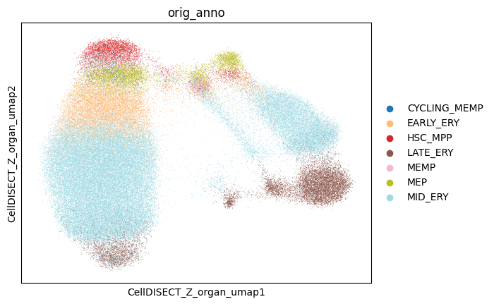
[16]:
fig, ax = plt.subplots(nrows=1, ncols=1)
sc.pl.embedding(
    adata,
    basis='CellDISECT_Z_organ_umap',
    color='orig_anno',
    groups=celltypes,
    ax=ax,
    show=False,
    )
# fig.savefig('ery_figs/zOrgan_orig_anno.png', dpi=150, bbox_inches='tight')
# fig.savefig('ery_figs/zOrgan_orig_anno.svg', dpi=150, bbox_inches='tight')
# plt.show()
# plt.close(fig)
[16]:
<Axes: title={'center': 'orig_anno'}, xlabel='CellDISECT_Z_organ_umap1', ylabel='CellDISECT_Z_organ_umap2'>
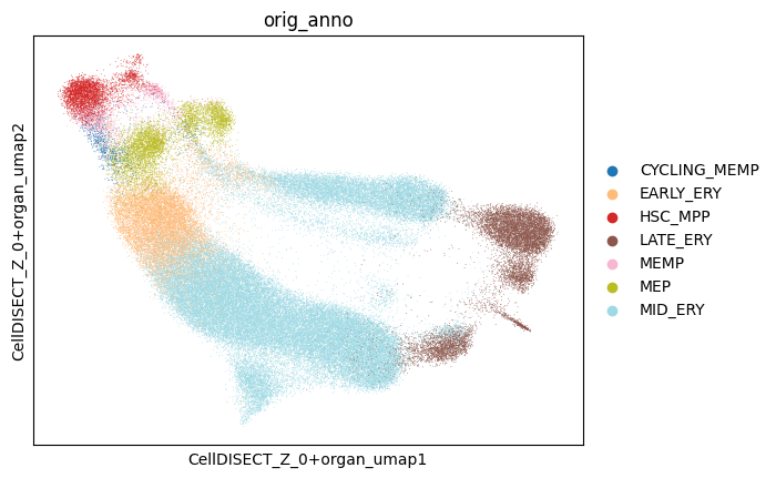
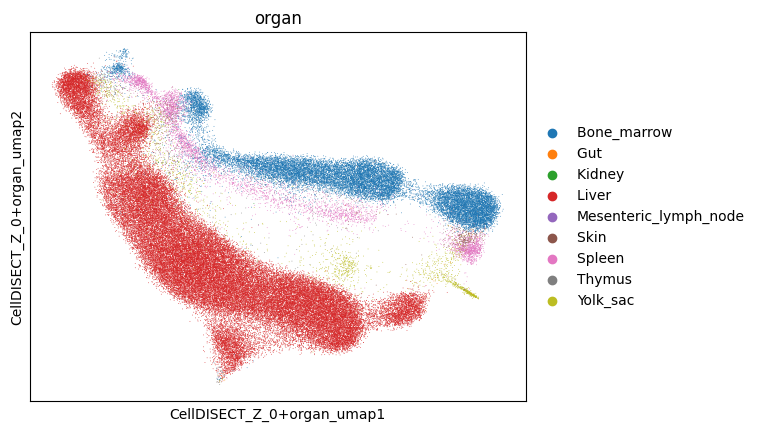
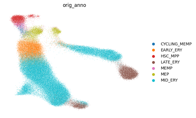
3.3.2. You can easily see the separation of different organs and cell types within one latent represantation (Z0+Organ) and you can analyse the different clusters
[17]:
fig, ax = plt.subplots(nrows=1, ncols=1)
sc.pl.embedding(
    adata, basis='CellDISECT_Z_0+organ_umap', color='orig_anno', groups=celltypes,
    ax=ax,
    show=False,
    )
# fig.savefig('ery_figs/zOrgan+0_orig_anno.png', dpi=150, bbox_inches='tight')
# fig.savefig('ery_figs/zOrgan+0_orig_anno.svg', dpi=150, bbox_inches='tight')
# plt.show()
# plt.close(fig)
[17]:
<Axes: title={'center': 'orig_anno'}, xlabel='CellDISECT_Z_0+organ_umap1', ylabel='CellDISECT_Z_0+organ_umap2'>
[18]:
fig, ax = plt.subplots(nrows=1, ncols=1)
sc.pl.embedding(
    adata, basis='CellDISECT_Z_0+organ_umap', color='organ',
    ax=ax,
    show=False,
    )
# fig.savefig('ery_figs/zOrgan+0_organ.png', dpi=150, bbox_inches='tight')
# fig.savefig('ery_figs/zOrgan+0_organ.svg', dpi=150, bbox_inches='tight')
# plt.show()
# plt.close(fig)
[18]:
<Axes: title={'center': 'organ'}, xlabel='CellDISECT_Z_0+organ_umap1', ylabel='CellDISECT_Z_0+organ_umap2'>
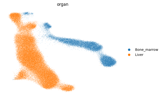
3.4. Now we want to take a closer look at Liver and Bone Marrow cells
[19]:
adata = adata[adata.obs['organ'].isin(['Liver ', 'Bone_marrow '])].copy()
adata
[19]:
AnnData object with n_obs × n_vars = 82585 × 8192
    obs: 'study', 'sample_ID', 'lane_ID', 'organ', 'age', 'cell_type', 'sex', 'sex_inferred', 'sample_status', 'library_platform', 'strand_sequence', 'biological_unit', 'doi', 'institute', 'study_PI', 'subject_ID', 'ethnicity_1', 'ethnicity_2', 'disease_known', 'disease_condition', 'subject_type', 'sample_type', 'sample_cultured', 'anatomical_region', 'anatomical_region_level_2', 'protocol_tissue_dissociation', 'cell_enrichment', 'reference_genome', 'reference_genome_ensembl_release', 'reads_processing', 'sequencing_platform', 'Sample_orig_author', 'Anatomical_region_orig_author', 'Termination_method_orig_author', 'Method_orig_author', 'anno_lvl_2_final_clean_orig_author', 'integration_donor', 'integration_biological_unit', 'integration_sample_status', 'integration_library_platform_coarse', 'author_batch', 'Chuan_meta_Original_Label', 'Chuan_meta_Harmonised_Label', 'Chuan_meta_Tissue', 'Chuan_meta_Technology', 'Chuan_meta_Donor', 'Chuan_meta_Age', 'orig_anno', 'trimester', 'bin_age', '_cluster', '_scvi_batch', '_scvi_labels', '_scvi_cluster'
    var: 'GeneID', 'GeneName', 'n_counts', 'highly_variable', 'means', 'dispersions', 'dispersions_norm'
    uns: '_scvi_manager_uuid', '_scvi_uuid', 'bin_age_colors', 'cell_type_colors', 'hvg', 'integration_donor_colors', 'integration_library_platform_coarse_colors', 'log1p', 'organ_colors', 'CellDISECT_Z_0_neighbors', 'CellDISECT_Z_organ_neighbors', 'CellDISECT_Z_0+organ_neighbors', 'orig_anno_colors'
    obsm: '_scvi_extra_categorical_covs', 'CellDISECT_Z_0', 'CellDISECT_Z_integration_donor', 'CellDISECT_Z_not_integration_donor', 'CellDISECT_Z_integration_library_platform_coarse', 'CellDISECT_Z_not_integration_library_platform_coarse', 'CellDISECT_Z_organ', 'CellDISECT_Z_not_organ', 'CellDISECT_Z_0+integration_donor', 'CellDISECT_Z_0+integration_library_platform_coarse', 'CellDISECT_Z_0+organ', 'CellDISECT_Z_0_organ_integration_donor', 'CellDISECT_Z_0_umap', 'CellDISECT_Z_organ_umap', 'CellDISECT_Z_0+organ_umap'
    layers: 'counts'
3.4.1. We recompute the neighbors for this subset
[20]:
anno_col = 'orig_anno'
latent = 'CellDISECT_Z_0+organ'

sc.pp.neighbors(adata, n_neighbors=15, use_rep=latent)
sc.tl.umap(adata)
[21]:
fig, ax = plt.subplots(nrows=1, ncols=1)
sc.pl.umap(
    adata,
    color=anno_col,
    palette='tab10',
    frameon=False,
    ax=ax,
    show=False,
    )
# fig.savefig('ery_figs/subset_zrgan+0_organ.png', dpi=150, bbox_inches='tight')
# fig.savefig('ery_figs/subset_zrgan+0_organ.svg', dpi=150, bbox_inches='tight')
# plt.show()
# plt.close(fig)
[21]:
<Axes: title={'center': 'orig_anno'}, xlabel='UMAP1', ylabel='UMAP2'>
[37]:
fig, ax = plt.subplots(nrows=1, ncols=1)
sc.pl.umap(
    adata,
    color='organ',
    frameon=False,
    ax=ax,
    show=True,
    )
# fig.savefig('ery_figs/subset_zrgan+0_organ.png', dpi=150, bbox_inches='tight')
# fig.savefig('ery_figs/subset_zrgan+0_organ.svg', dpi=150, bbox_inches='tight')
# plt.show()
# plt.close(fig)
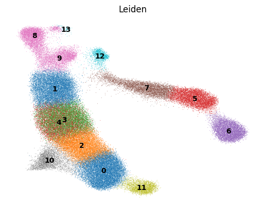
[22]:
sc.tl.leiden(adata, key_added='Leiden', resolution = 2)
sc.pl.umap(adata, color='Leiden')
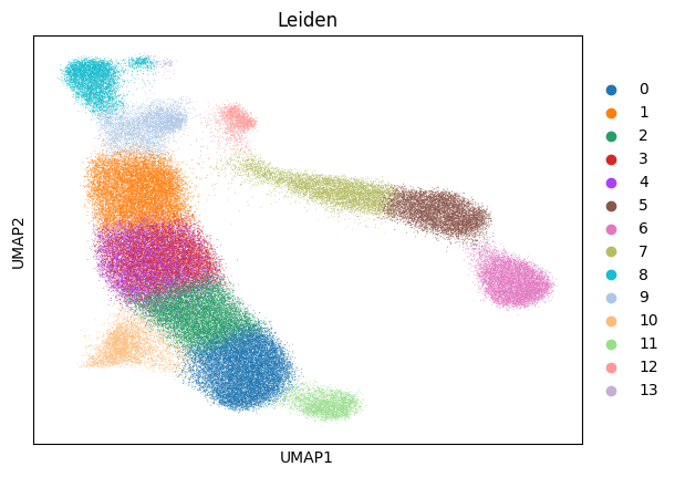
[23]:
fig, ax = plt.subplots(nrows=1, ncols=1)
sc.pl.umap(adata, color='Leiden', legend_loc = 'on data',
    palette='tab10',
    frameon=False,
    ax=ax,
    show=False,
    )
# fig.savefig('ery_figs/subset_zrgan+0_leiden.png', dpi=150, bbox_inches='tight')
# fig.savefig('ery_figs/subset_zrgan+0_leiden.svg', dpi=150, bbox_inches='tight')
# plt.show()
# plt.close(fig)
[23]:
<Axes: title={'center': 'Leiden'}, xlabel='UMAP1', ylabel='UMAP2'>